Agentic variant analysis of the 1000 Genomes Project using Polars, DuckDB, and lakehouses  

The 1000 Genomes Project sequenced 3202 individuals worldwide to build a comprehensive atlas of human genetic variation. Here, we discuss how to efficiently analyze 100M+ genomic variants in the age of agents. We evaluate modern query engines like Polars and DuckDB for streaming these large, distributed datasets, and show how lakehouse frameworks (Iceberg, LanceDB, LaminDB) address the efficiency and integrity problems of letting agents interact directly with raw files.
An atlas like 1000 Genomes[1] serves as a foundational reference for researchers to understand disease-associated mutations and evolutionary history. Such studies often require querying large amounts of data and are increasingly performed by AI agents leveraging formats such as Parquet. Several benchmarks show that queries of Parquet files can be up to 1000x faster than querying VCF files, not to mention the advantages of cloud-native access.[2][3][4][5] Hence, we transform two collections of VCF files to Parquet files:
# |
Pipeline |
Variant types |
Grouping |
Variants |
Files |
Source |
Explore |
|---|---|---|---|---|---|---|---|
1 |
DRAGEN[6] |
CNVs |
Per-individual |
4.86M |
3201 |
||
2 |
EMBL SHAPEIT2[7] |
CNVs, SNVs, Indels |
Per-chromosome |
88M |
26 |
The first collection stores individual-level information—such as the individual’s identifier, their specific genotype call, and the length of the structural variant. The second dataset is a population-level catalog of all unique variants, recording the location, type, and both global and population-specific allele frequencies.
Data access
Modern query engines like Polars[8] and DuckDB[9] vastly outperform classical data access methods, yet these formidable tools are often pointed at raw file storage systems or data lakes.
In these environments, the relevant .vcf and .parquet files are often buried within massive collections of mixed file types. While AI agents can navigate these storage systems, doing so forces them to waste tokens simply finding files and verifying their schemas.
A recent study[10] demonstrated that agents can fail entirely when accessing data across heterogeneous sources, but succeed when provided with a unified schema or API layer.
A simple agentic analysis
To illustrate this, we tasked an agent with a simple analysis: determine the number and types of variants in a specific genomic band. This mimics a typical workflow where researchers zoom into a specific genomic region or locus to study local variants, for instance, to identify mutations linked to a specific disease gene or to prepare data for a genome-wide association study (GWAS) focused on a candidate region. If the data was in a single DataFrame df, the analysis would look like this using the polars Python package:
import polars as pl

# filter variants
chrom = "1"
lo, hi = 150_000_000, 200_000_000
filtered = df.filter(
    (pl.col("chrom") == chrom) & (pl.col("pos") >= lo) & (pl.col("pos") <= hi)
).collect()

# breakdown by variant type, for context
by_type = (
    filtered.group_by("variant_type")
    .agg(pl.len().alias("n"))
    .sort("n", descending=True)
    .collect()
)
But it’s not. Hence, an agent first needs to find the files, and once it finds them, it needs to investigate whether they have the same schema so that they can be efficiently queried. So, it runs something like this:
# find files with a consistent schema
schemas, valid_filepaths = [], []
for filepath in filepaths:
    schema = pl.scan_parquet(filepath).collect_schema()
    if not schemas or schema == schemas[0]:
        schemas.append(schema)
        valid_filepaths.append(filepath)

# create a dataframe from files with a consistent schema
df = pl.scan_parquet(valid_filepaths)
To make things easy for the agent, let’s test it on Dataset 2 – which is distributed across just 26 files rather than 3200. We also prompt the agent with the exact file paths to spare it the trouble of finding them. Even with this head start, the agent still burns significant time and tokens just navigating files and checking schemas (Figure 1).
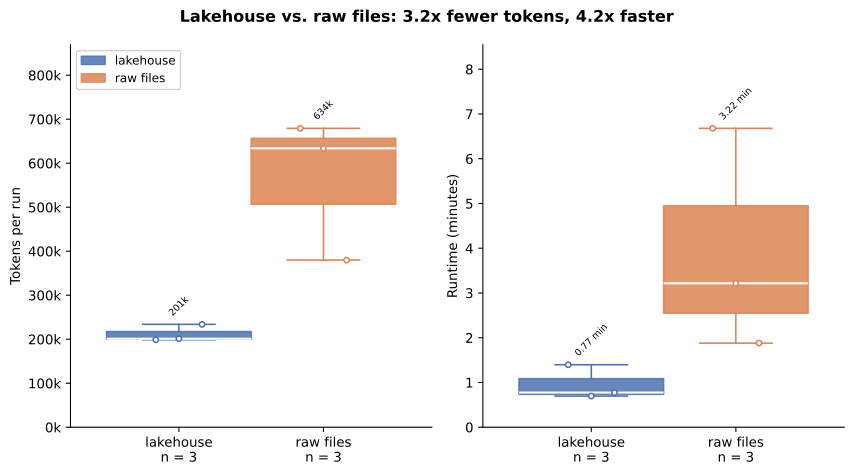
Figure 1 (source): Tokens and time required for an agent (Claude Code with claude-opus-5[1m]) to analyze variants across a genomic region using Polars on Dataset 2 (26 files). Compare an exemplary agent run on raw files against a run that leverages the schema contract of a collection.
A schema contract
Now, what if the 26 files formed one dataset together? An agent could trust that all files have a consistent schema and start deriving queries, and it wouldn’t even need to navigate filepaths. Fortunately, this is one problem that all lakehouses solve: they present a collection of parquet files as a single table to the user. We’ll deep dive on different lakehouse frameworks later, but here is how the access pattern looks with LaminDB:
import lamindb as ln

# Connect to the database
db = ln.DB("laminlabs/1000genomes")

# Retrieve the collection
collection = db.Collection.get("hVu9puwdRGskm1I6")

# Confirm the schema contract for these files
collection.schema.describe()

# Open the collection as a lazy Polars dataframe
df = collection.open(engine="polars")
The schema contract for the 26 parquet files can also be visualized, showing the 12 features computed in the EMBL SHAPEIT2 pipeline[7] (Figure 2).
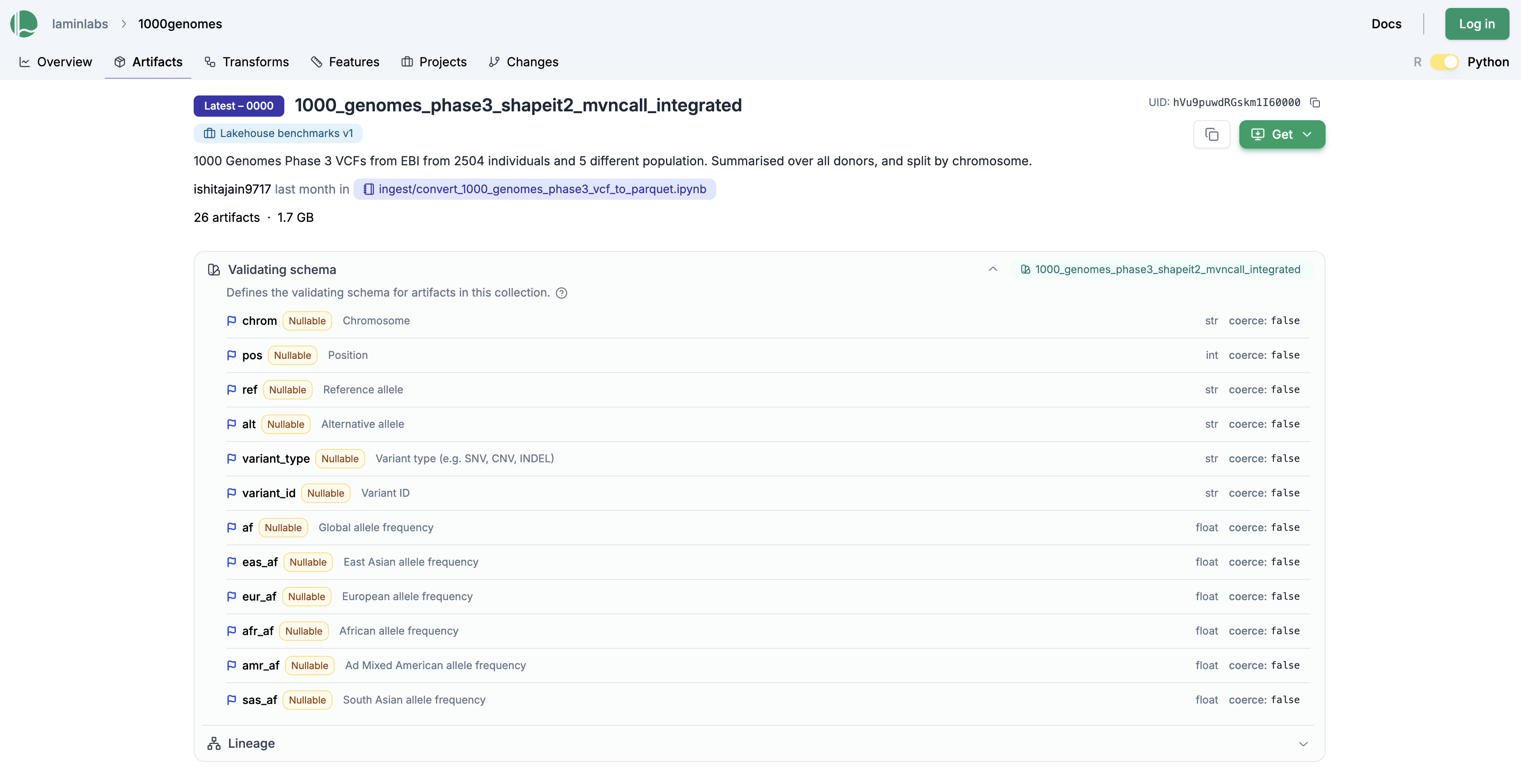
Figure 2: Screenshot of Dataset 2 with descriptions of its features.
The result is an agentic analysis that costs 3x fewer tokens and is 4x faster (Figure 1), with a comparable prompt and the same context. While ensuring efficient data access has a big impact on agentic efficiency and is often equated to “AI-ready data”, it’s little help if the actual data queries are inefficient. Let’s put them to the test!
Queries
We will be using the popular query engines Polars,[8] DuckDB,[9] and PyArrow,[11] all of which handle datasets that don’t fit into memory by streaming them directly from storage. It is worth noting that a new generation of readers can also efficiently query raw .vcf files directly.[12] However, they lack the advantages of cloud nativeness and a much broader big data ecosystem, and hence we’ll not study them in this post.
Simple filter
Let us first look at the simple filter from the analysis above across all three query engines:
with collection.open(engine="polars") as df:
    filtered = df.filter(
        (pl.col("CHROM") == chrom) & (pl.col("POS") >= lo) & (pl.col("POS") <= hi)
    ).collect()
import pyarrow.compute as pc

with collection.open(engine="pyarrow") as dataset:
    expr = ((pc.field("CHROM") == chrom)
            & (pc.field("POS") >= lo) & (pc.field("POS") <= hi))
    filtered = dataset.to_table(filter=expr)
To query via DuckDB, we need to register a lazy view over the collection’s S3 paths. The source bucket is cross-account (EU), so credentials are extracted from the artifact’s own storage session — PROVIDER credential_chain does not authenticate here. Creating this view takes around 40 sec for Dataset 1 and 3 sec for Dataset 2.
import duckdb
con = duckdb.connect()
con.execute("INSTALL httpfs; LOAD httpfs;")

# extract frozen session-token credentials from the artifact's storage session
# (see duckdb_pipeline.ipynb for the full async extraction)
con.execute(f"""
    CREATE OR REPLACE SECRET s3 (
        TYPE s3, KEY_ID '{access_key}', SECRET '{secret_key}',
        SESSION_TOKEN '{token}', REGION 'eu-central-1'
    )
""")

s3_paths = [a.path.as_posix() for a in collection.artifacts.all()]
con.execute(f"CREATE OR REPLACE VIEW cnv_vcf AS SELECT * FROM read_parquet({s3_paths})")
The actual query is then:
filtered = con.execute(
    "SELECT * FROM cnv_vcf WHERE CHROM = ? AND POS BETWEEN ? AND ?",
    [chrom, lo, hi],
).df()
Summary statistics
Profiling summary statistics is a standard exploratory step to assess genetic diversity, establish baselines for rare disease studies, and identify severe structural variations before downstream association studies. Here, we calculate the total CNV count, deletions, median deletion size, and homozygous/heterozygous counts:
stats = (
    df.group_by("SAMPLE_NAME").agg(
        pl.len().alias("Total_CNVs"),
        (pl.col("INFO_SVLEN") < 0).sum().alias("Deletions"),
        pl.col("INFO_SVLEN").filter(pl.col("INFO_SVLEN") < 0).abs().median().alias("Median_Deletion_Size"),
        (pl.col("SAMPLE_GT") == "1/1").sum().alias("Homozygous_CNVs"),
        (pl.col("SAMPLE_GT") == "0/1").sum().alias("Heterozygous_CNVs"),
    ).sort("SAMPLE_NAME").collect()
)
# Native PyArrow aggregation. Note: PyArrow only offers an *approximate* (t-digest)
# grouped median, so Median_Deletion_Size is approximate for PyArrow; SQL/Polars are exact.
t = dataset.to_table(columns=["SAMPLE_NAME", "INFO_SVLEN", "SAMPLE_GT"])
t = t.append_column("is_del", pc.cast(pc.less(t["INFO_SVLEN"], 0), pa.int64()))
t = t.append_column("is_hom", pc.cast(pc.equal(t["SAMPLE_GT"], "1/1"), pa.int64()))
t = t.append_column("is_het", pc.cast(pc.equal(t["SAMPLE_GT"], "0/1"), pa.int64()))
base = t.group_by("SAMPLE_NAME").aggregate([
    ("SAMPLE_NAME", "count"), ("is_del", "sum"), ("is_hom", "sum"), ("is_het", "sum"),
])
dels = t.filter(pc.less(t["INFO_SVLEN"], 0))
dels = dels.append_column("abs_svlen", pc.abs(dels["INFO_SVLEN"]))
med = dels.group_by("SAMPLE_NAME").aggregate([("abs_svlen", "approximate_median")])
stats = base.join(med, keys="SAMPLE_NAME", join_type="left outer")
stats = con.execute("""
    SELECT SAMPLE_NAME,
           COUNT(*)                                              AS Total_CNVs,
           COUNT(*) FILTER (WHERE INFO_SVLEN < 0)                AS Deletions,
           MEDIAN(ABS(INFO_SVLEN)) FILTER (WHERE INFO_SVLEN < 0) AS Median_Deletion_Size,
           COUNT(*) FILTER (WHERE SAMPLE_GT = '1/1')             AS Homozygous_CNVs,
           COUNT(*) FILTER (WHERE SAMPLE_GT = '0/1')             AS Heterozygous_CNVs
    FROM cnv_vcf
    GROUP BY SAMPLE_NAME
""").df()
Recurrent regions
Finding recurrent mutation hotspots helps pinpoint highly mutable regions, functional genomic elements under evolutionary pressure, and common structural variations across populations. To identify these, we bin positions into genomic windows (1 kbp for Dataset 1, 1 Mbp for Dataset 2) and flag bins containing variants from multiple samples.
recurrent = (
    df.with_columns(
        (pl.col("CHROM").cast(pl.Utf8) + ":" +
         ((pl.col("POS") // 1000) * 1000).cast(pl.Utf8)).alias("region_key")
    )
    .group_by("region_key").agg(pl.col("SAMPLE_NAME").n_unique().alias("sample_count"))
    .filter(pl.col("sample_count") >= 2)
    .sort("sample_count", descending=True).collect()
)
t = dataset.to_table(columns=["CHROM", "POS", "SAMPLE_NAME"])
bin_start = pc.multiply(pc.cast(pc.divide(t["POS"], 1000), pa.int64()), 1000)
region_key = pc.binary_join_element_wise(
    pc.cast(t["CHROM"], pa.string()), pc.cast(bin_start, pa.string()), ":")
t = t.append_column("region_key", region_key)
pairs = t.select(["region_key", "SAMPLE_NAME"]).group_by(["region_key", "SAMPLE_NAME"]).aggregate([])
counts = pairs.group_by("region_key").aggregate([("SAMPLE_NAME", "count")])
recurrent = counts.filter(pc.greater_equal(counts["SAMPLE_NAME_count"], 2))
recurrent = con.execute("""
    SELECT CHROM || ':' || CAST((POS // 1000) * 1000 AS VARCHAR) AS region_key,
           COUNT(DISTINCT SAMPLE_NAME) AS sample_count
    FROM cnv_vcf
    GROUP BY region_key
    HAVING COUNT(DISTINCT SAMPLE_NAME) >= 2
    ORDER BY sample_count DESC
""").df()
Timing results
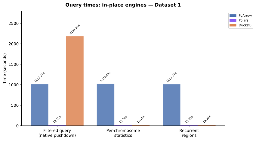
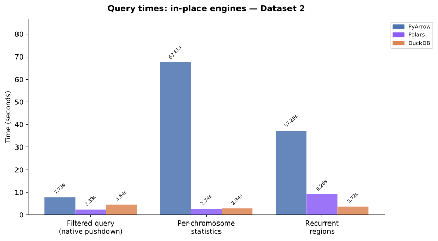
Benchmarking these queries reveals two major takeaways (Figure 3):
First, Polars is the only query engine that efficiently handles the massive file count (3,201 files) of Dataset 1. Because DuckDB cold-reads Parquet files over httpfs, it is bottlenecked by 3,201 sequential S3 footer round-trips just to locate row groups. This explains why DuckDB is dramatically slower here, despite Dataset 1 having 20x fewer rows than Dataset 2.
Second, while Polars delivers the fastest query times overall, DuckDB pulls ahead on complex relational logic—specifically, the recurrent region detection in Dataset 2.
Data management
Working with a high number of raw files across different sources almost inevitably leads to fragile data organization. This brittleness is amplified when working with agents: they prioritize solving the immediate task over long-term maintainability, they make frequent mistakes, and their concurrent read/write patterns can quickly corrupt a purely file-based architecture. Lakehouse frameworks solve these problems with ACID transactions to prevent partial writes, with schema enforcement to prevent inconsistent datasets, and with time travel to easily restore erroneous written datasets. And, as discussed earlier, they also make agents more efficient. So, let’s briefly review available options.
Frameworks
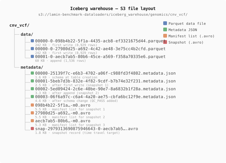 Figure 4. File layout of an Iceberg table.
Today’s most popular framework is Iceberg.[13] Like Delta Lake[14][15] and Apache Hudi,[16] Iceberg provides ACID transactions and “time travel” by organizing parquet files into snapshots, managed by manifest and metadata files (Figure 4). However, this file-based metadata introduces costs (snapshot creation is expensive dictating large, infrequent writes), optimistic concurrency leads to conflicts between simultaneous writers, and coordinating updates on S3 requires an external catalog like AWS Glue or Nessie.[17]
Feature |
Raw S3 |
Iceberg |
DuckLake |
LaminDB |
|---|---|---|---|---|
Data lake (file management & annotation) |
✅ |
❌ |
❌ |
✅ |
ACID transactions |
❌ |
✅ |
✅ |
✅ ¹ |
Time travel / snapshot version isolation |
❌ |
✅ |
✅ |
✅ ² |
Schema evolution without rewriting data |
❌ |
✅ ³ |
✅ ³ |
✅ ³ |
Write-Audit-Publish workflow |
❌ |
✅ |
❌ |
✅ ⁴ |
Query engine independence |
✅ |
✅ |
❌ |
✅ |
Concurrent writers |
❌ ⁵ |
❌ |
✅ |
✅ |
Automatic maintenance |
❌ |
❌ |
✅ ⁶ |
✅ ⁶ |
Native multi-table transactions |
❌ |
❌ |
✅ |
❌ |
Dataset formats beyond tables |
✅ |
❌ |
❌ |
✅ |
Data lineage |
❌ |
❌ |
❌ |
✅ |
Registries/ontologies |
❌ |
❌ |
❌ |
✅ |
Table 1. A high-level overview of lakehouse technologies.
¹ LaminDB guarantees data ↔ metadata consistency through ACID operations, but does not guarantee row-level ACID operations the way Iceberg and DuckLake do. Because you can map an insert into a collection of parquet files via lamindb.Collection.append() in an ACID way, the practical robustness guarantee to the user is similar.
² See the Developer experience section for examples.
³ Adding a nullable/optional column without rewriting existing files.
⁴ In LaminDB, via branches (stage, review, merge).
⁵ Raw files have no commit protocol; concurrent writers risk partial writes / last-writer-wins.
⁶ No need for cleaning orphaned files like in Iceberg.
An increasingly popular approach to addressing Iceberg’s limitations is DuckLake,[18][19] developed by the DuckDB team. Rather than storing metadata in files, DuckLake keeps all metadata in a relational database, leaving only parquet files in storage. This gives it cheap writes that can be more frequent, transactions with true concurrent writer support, automatic maintenance via the database’s native mechanisms, and native multi-table transactions — all things that are difficult or impossible with Iceberg’s file-based metadata.
Unlike Iceberg and DuckLake, LaminDB goes beyond tables, supporting datasets across any storage format — Parquet, AnnData, HDF5, Zarr, VCF, and more. The user can manage anything from blobs in a data lake to multimodal datasets based on a single schema concept. LaminDB shares DuckLake’s architectural design — a relational database for metadata and storage for data — and natively provides data lineage (Table 1).
While Iceberg & DuckLake are based on the parquet format, and LaminDB is format-agnostic, LanceDB manages datasets in the Lance format, a columnar format inspired by parquet that’s optimized for arrays.[20] To use LanceDB, you need to convert your data into the Lance format.
While LanceDB fits the lakehouse architecture, non-lakehouse architectures for managing array-like data exist, too, in particular, arraylake & tensorstore for .zarr arrays, and tiledb for .tiledb arrays.[21] These non-lakehouse technologies are out of scope for this post given the established query engines don’t apply to them.
Developer experience
To see how these concepts translate into developer experience, let’s compare the code required to perform these essential agentic operations—appending data, evolving schemas, and time-traveling. In the queries themselves, there is no noteworthy difference to what we’ve discussed above (see Querying Iceberg & LanceDB).
The first type of write operation we need to perform is adding new data to the system. Rather than just dropping a raw file into a bucket, the following code snippets ensure that a new dataset complies with the schema of the existing dataset, and that it’s added in an ACID fashion.
Atomic and snapshot-isolated. New Parquet files and a snapshot manifest are written to S3; concurrent readers see a consistent state throughout.
table.append(batch) # batch is a pyarrow dataset
add() writes new rows to S3 and automatically increments the table version.
table.add(batch) # batch is a pyarrow dataset
Atomic and snapshot-isolated. A new parquet file creates a new collection version.
collection.append(batch) # batch is an artifact
Similarly, when an analysis requires new features, the following snippets ensure that columns are updated consistently across the entire dataset, and future incoming datasets.
A new metadata file records the updated schema. Existing Parquet files are not modified; reads of old files return null for the new column.
from pyiceberg.types import BooleanType
with table.update_schema() as update:
    update.add_column("QC_PASS", BooleanType())
add_columns takes a per-column SQL value expression — hence the CAST(NULL AS BOOLEAN) string, which supplies both the value and its type for existing rows.
table.add_columns({"QC_PASS": "CAST(NULL AS BOOLEAN)"})
LaminDB registers the feature in its schema registry, validating all future artifacts instance-wide.
feature = ln.Feature(name="QC_PASS", dtype=bool).save()
collection.schema.add(feature)
Finally, because agents inevitably make mistakes, we look at how to retrieve a previous version of a dataset via “time travel”.
first_snapshot = table.history()[0].snapshot_id  # access version 0
table.scan(snapshot_id=first_snapshot)
table.checkout(1) # checkout a previous version
collection.versions.get(version="1") # get a previous version
The age of agents is transforming how we interact with large biological datasets like the 1000 Genomes Project. However, as our benchmarks show, pairing highly capable query engines (like Polars and DuckDB) with disorganized data lakes creates an immediate bottleneck: agents waste compute finding files and guessing schemas, and they corrupt data with concurrent writes and poor choices. By evolving the underlying data architecture from mere storage systems to lakehouse frameworks, one can provide agents with the ACID guarantees, schema enforcement, and unified access they need to operate safely and efficiently at scale.
Code & data availability
The datasets, the agentic analyses, the queries, the shared benchmarking utilities, and the plotting script are available in the public laminlabs/1000genomes database. They can be browsed through data lineage by clicking on the “source” link in every figure caption.
Methods
Dataset curation
Dataset 1 (lineage): The 1000 Genomes Project datasets were sourced from the Registry of Open Data on AWS, specifically the DRAGEN v3.7.6 reanalysis (s3://1000genomes-dragen). For Dataset 1, we read the .cnv.vcf.gz files directly from the S3 bucket into memory using pysam, flattened the VCF records (including nested INFO and FORMAT fields) into a tabular structure, and saved them to LaminDB as partitioned Parquet files (.cnv.parquet). You can trace the run here.
Note that while the full high-coverage expanded cohort of the 1000 Genomes Project contains 3,202 individuals, the DRAGEN hg38 reanalysis we pulled from contains exactly 3,201 files. This is because one sample (NA18498) from the original Phase 3 release was excluded during the re-alignment to the GRCh38 reference genome, a common occurrence in genomics due to relatedness discoveries or quality control thresholds.
Dataset 2 (lineage): The Phase 3 release of the 1000 Genomes Project is one of the most comprehensive dataset from the original project, comprising whole-genome and exome sequencing data from 2,504 individuals across 26 populations spanning 5 continental populations (AFR, AMR, EAS, EUR, SAS). Variant calls are provided as VCF files, split per chromosome, with the standard naming convention. Each field in the filename encodes one step of the pipeline, in order — ALL (cohort) → chr<N> (which chromosome the file covers) → phase3 (release/call-set version) → shapeit2_mvncall_integrated (methods used, in the order applied: MVNCall integrates calls, then SHAPEIT2 phases them) → 20130502 (release date, YYYYMMDD).
Query timings
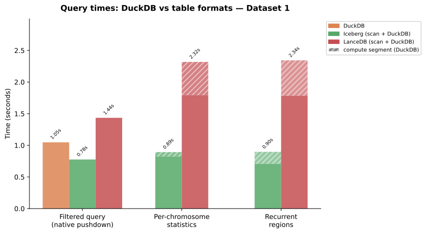
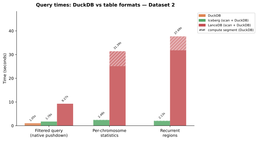
All timings are single-run measurements on SageMaker (ml.m5.24xlarge) in store mode. Versions: lamindb-core==2.7.0, duckdb==1.5.3, polars==1.42.0, pyiceberg==0.11.1, lancedb==0.33.0, pandas==2.3.3, Python 3.12. Query engines (PyArrow, Polars, DuckDB) compute natively; table formats (Iceberg, LanceDB) scan natively and aggregate in DuckDB. PyArrow’s grouped median is approximate (t-digest); the others are exact. Because the two datasets differ in schema, Queries 2 and 3 run analogous but not identical analyses (per-sample on Dataset 1, per-chromosome on Dataset 2); the read and filter operations are identical in logic across datasets and carry the file-count comparison. Single-run numbers are point measurements, not distributions.
Querying Iceberg & LanceDB
This section demonstrates that there isn’t a noteworthy difference in querying parquet files, the Iceberg, or the LanceDB format. To study the latter, we have to convert parquet files into the Iceberg and LanceDB table formats.
from pyiceberg.catalog.sql import SqlCatalog

arrow = collection.open().to_table()
catalog = SqlCatalog("local", uri="sqlite:///iceberg_catalog.db", warehouse=WAREHOUSE)
catalog.create_namespace("genomics")
table = catalog.create_table("genomics.cnv_vcf", schema=arrow.schema)
table.append(arrow)
import lancedb

arrow = collection.open().to_table()
db = lancedb.connect(WAREHOUSE)
table = db.create_table("cnv_vcf", data=arrow, mode="overwrite")
The timing results for format conversion are dominated by the conversion to a PyArrow dataset, and take substantially longer for LanceDB than for Iceberg for the larger Dataset 2.
Operation |
Dataset |
Iceberg (sec) |
LanceDB (sec) |
|---|---|---|---|
Read |
1 |
2043 |
2045 |
Read |
2 |
43 |
45.2 |
Ingest |
1 |
6 |
7 |
Ingest |
2 |
5.7 |
109 |
Query 1. Because the format conversion implies a much lower number of files for Iceberg and LanceDB, we’re also converting the original parquet files to a single parquet file, so that we’re not biasing performance of Query 1 due to the high number of files.
path = db.Artifact.get(key="benchmark/dragen_cnv.parquet").path.as_posix()
duckdb.sql(f"""
    SELECT "Chromosome", count(*) AS n_calls
    FROM read_parquet('{path}')
    WHERE "QUAL" >= 30
    GROUP BY "Chromosome"
    ORDER BY n_calls DESC
""").show()
from pyiceberg.expressions import And, EqualTo, GreaterThanOrEqual, LessThanOrEqual
row_filter = And(EqualTo("CHROM", chrom),
             And(GreaterThanOrEqual("POS", lo), LessThanOrEqual("POS", hi)))
filtered = table.scan(row_filter=row_filter).to_arrow()
# .to_lance() exposes the underlying Lance dataset so the predicate pushes down
# at the storage layer; the LanceDB table wrapper doesn't expose that filter directly.
filtered = table.to_lance().to_table(
    filter=f"CHROM = '{chrom}' AND POS BETWEEN {lo} AND {hi}"
)
Query 2 & 3. Both of these queries cannot be natively run via pyiceberg or lancedb. Hence, we’re timing results for a DuckDB-based query after converting back from pyarrow.
# Iceberg is a table format, not a compute engine: native scan, then aggregate in DuckDB.
arrow = table.scan().to_arrow()
stats = compute_duckdb(arrow, SQL_EXPRESSION)
arrow = table.to_arrow()
stats = compute_duckdb(arrow, SQL_EXPRESSION)
How is compute_duckdb processing information
def compute_duckdb(arrow_table, sql):
    """Format already scanned natively; run the standard aggregation in DuckDB."""
    con = duckdb.connect()
    con.register("t", arrow_table)
    return con.execute(sql.format(src="t")).df()
How to cite
Pillai R, Rasmussen A, Jain I, Sun S, Rybakov S & Wolf A (2026). Agentic variant analysis of the 1000 Genomes Project using Polars, DuckDB, and lakehouses. Lamin Blog. https://blog.lamin.ai/1000genomes